Tag: Polars

  • Leveraging Scikit-Learn and Polars to Test a Naive Bayes Classifier

    Leveraging Scikit-Learn and Polars to Test a Naive Bayes Classifier

    In today’s post, I use scikit-learn with the same sample dataset I used in the previous post. I need to use the LabelEncoder to encode the strings as numeric values and then the GaussianNB to train and testing a Gaussian Naive Bayes classifier model and to predict the class of an example record. While many tutorials use pandas, I use Polars for fast data manipulation alongside scikit-learn for model development.

    Understanding Our Data and Tools

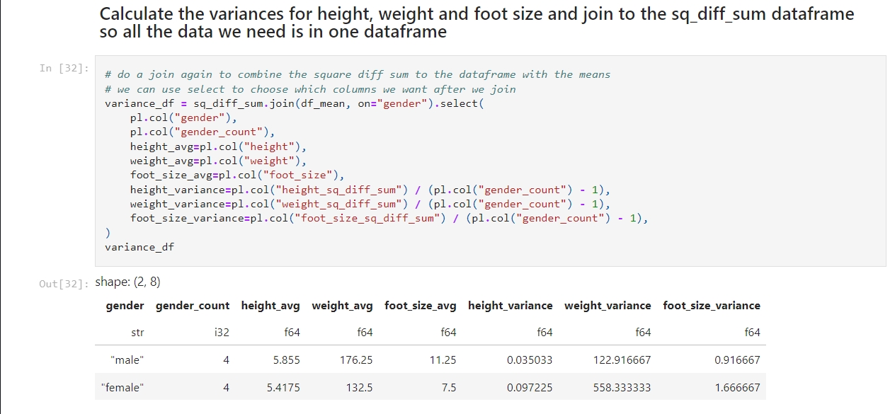
    Remember that the dataset includes ‘features’ for height, weight, foot size. It also has a categorical field for gender. Because classifiers like Gaussian Naive Bayes require numeric inputs, I need to transform the string gender values into a numeric format.

    In my new Jupyter notebook I use two libraries:

    Scikit-Learn for its machine learning utilities. Specifically, LabelEncoder for encoding and GaussianNB for classification.

    Polars for fast, efficient DataFrame manipulations.

    Step 1: Encoding Categorical Variables

    The first step is to convert our categorical column (gender) to a numeric format using scikit-learn’s LabelEncoder. This conversion is vital because machine learning models generally can’t work directly with string labels.

    Below is the code from our first notebook cell:

    In that cell:

    • I instantiate a LabelEncoder object.
    • For every feature in columns_to_encode (in this case, just "gender"), I create a new Polars Series with the suffix "_num", containing the encoded numeric values.
    • Finally, I add these series as new columns to our original DataFrame.

    This ensures that our categorical data is transformed into a machine-friendly format, an also preserves the human-readable string values for future reference.

    Step 2: Mapping Encoded Values to Original Labels

    Once we’ve encoded the data, it’s important to retain the mapping between the original string values and their corresponding numeric codes. This mapping is particularly useful when you want to interpret or display the model’s predictions.

    The following code block demonstrates how to generate and view this mapping:

    In that cell:

    • I save the original "gender" column and its encoded counterpart "gender_num".
    • By grouping on "gender" and aggregating with the first encountered numeric value, I create a mapping from string labels to numerical codes.

    Step 3: Training and Testing the Gaussian Naive Bayes Classifier

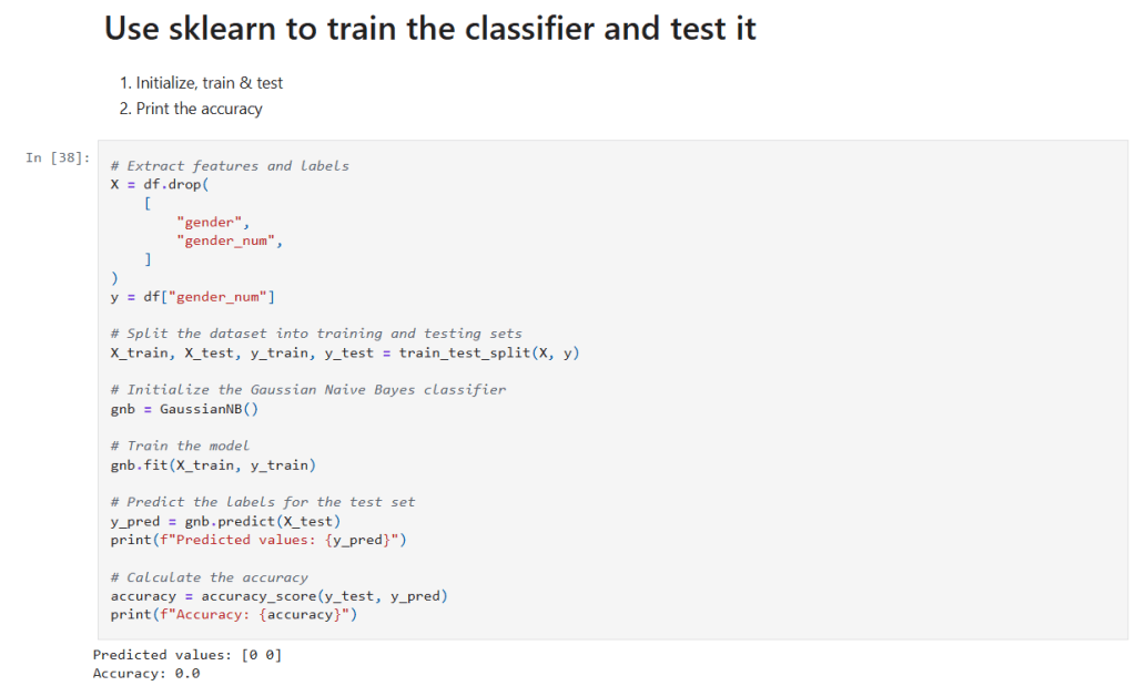
    Now it’s time to build, train, and evaluate our model. I separate the features and target, split the data, and then initialize the classifier.

    In that cell:

    • Get the data to use in training: I drop the raw "gender" and its encoded version from the Dataframe (X) and save the encoded classification in (y).
    • Data Splitting: train_test_split is used to randomly partition the data into training and testing sets.
    • Model Training: A GaussianNB classifier is instantiated and trained on the training data using the fit() method.
    • Prediction and Evaluation: The model’s predictions on the test set (y_pred) are generated and compared against the true labels using accuracy_score. This gives us a quantitative measure of the model’s performance.

    Step 4: Classifying a New Record

    Now I can test it on the sample observation. Consider the following code snippet:

    In that cell:

    • Create Example Data: I define a new sample record (with features like height, weight, and foot size) and create a Polars DataFrame to hold this record.
    • Prediction: The classifier is then used to predict the gender (encoded as a number) for this new record.
    • Decoding: Use the gender_mapping to display the human-readable gender label corresponding to the model’s prediction.

    Final Thoughts and Next Steps

    This step-by-step notebook shows how to preprocess data, map categorical values, train a Gaussian Naive Bayes classifier, and test new data with the combination of Polars and scikit-learn.

    The new Jupyter notebook can be found here in my GitHub. If you follow the instructions in my previous post you can run this notebook for yourself.

    – William

  • What I learned about the Gaussian Naive Bayes Classifier

    What I learned about the Gaussian Naive Bayes Classifier

    Description of Gaussian Naive Bayes Classifier

    Naive Bayes classifiers are simple supervised machine learning algorithms used for classification tasks. They are called “naive” because they assume that the features are independent of each other, which may not always be true in real-world scenarios. The Gaussian Naive Bayes classifier is a type of Naive Bayes classifier that works with continuous data. Naive Bayes classifiers have been shown to be very effective, even in cases where the the features aren’t independent. They can also be trained even with small datasets and are very fast once trained.

    Main Idea: The main idea behind the Naive Bayes classifier is to use Bayes’ Theorem to classify data based on the probabilities of different classes given the features of the data. Bayes’ Theorem says that we can tell how likely something is to happen, based on what we already know about something else that has already happened.

    Gaussian Naive Bayes: The Gaussian Naive Bayes classifier is used for data that has a continuous distribution and does not have defined maximum and minimum values. It assumes that the data is distributed according to a Gaussian (or normal) distribution. In a Gaussian distribution the data looks like a bell curve if it is plotted. This assumption lets us use the Gaussian probability density function to calculate the likelihood of the data. Below are the steps needed to train a classifier and then use to to classify a sample record.

    Steps to Calculate Probabilities (the hard way):

    1. Calculate the Averages (Means):
      • For each feature in the training data, calculate the mean (average) value.
      • To calculate the mean the sum of the values are divided by the number of values.
    2. Calculate the Square of the Difference:
      • For each feature in the training data, calculate the square of the difference between each feature value and the mean of that feature.
      • To calculate the square of the difference we subtract the mean from a value and square the result.
    3. Sum the Square of the Difference:
      • Sum the squared differences for each feature across all data points.
      • Calculating this is easy, we just add up all the squared differences for each feature.
    4. Calculate the Variance:
      • Calculate the variance for each feature using the sum of the squared differences.
      • We calculate the variance by dividing the sum of the squares of the differences by the number of values minus 1.
    5. Calculate the Probability Distribution:
      • Use the Gaussian probability density function to calculate the probability distribution for each feature.
      • The formula for this is complicated! It goes like this:
        • First take: 1 divided by the square root of 2 times pi times the variance.
        • Multiply that by e to the power of -1 times the square of the value to test minus the mean of the value divided by 2 times the variance.
    6. Calculate the Posterior Numerators:
      • Calculate the posterior numerator for each class by multiplying the prior probability of the class with the probability distributions of each feature given the class.
    7. Classify the sample data:
      • The higher result from #6 is the result.

    I created a Jupyter notebook that performs these calculations based on this example I found on Wikipedia. Here is my notebook on GitHub. If you follow the instructions in my previous post you can run this notebook for yourself.

    – William

    References

    1. Wikipedia contributors. (2025, February 17). Naive Bayes classifier. In Wikipedia, The Free Encyclopedia. Retrieved from https://en.wikipedia.org/wiki/Naive_Bayes_classifier
    2. Wikipedia contributors. (2025, February 17). Variance: Population variance and sample variance. In Wikipedia, The Free Encyclopedia. Retrieved from https://en.wikipedia.org/wiki/Variance#Population_variance_and_sample_variance
    3. Wikipedia contributors. (2025, February 17). Probability distribution. In Wikipedia, The Free Encyclopedia. Retrieved from https://en.wikipedia.org/wiki/Probability_distribution