

In today’s data-driven world, even seemingly straightforward questions can reveal surprising insights. In this post, I investigate whether students’ alcohol consumption habits bear any relationship to their final math grades. Using the Student Alcohol Consumption dataset from Kaggle, which contains survey responses on a myriad aspects of students’ lives—ranging from study habits and social factors to gender and alcohol use—I set out to determine if patterns exist that can predict academic performance.
Dataset Overview
The dataset originates from a survey of students enrolled in secondary school math and Portuguese courses. It includes rich, social, and academic information, such as:
- Social and family background
- Study habits and academic support
- Alcohol consumption details during weekdays and weekends
I focused on predicting the final math grade (denoted as G3 in the raw data) while probing how alcohol-related features, especially weekend consumption, might play a role in performance. The binary insight wasn’t just about whether students drank, but which drinking pattern might be more telling of their academic results.
Data Preprocessing: Laying the Groundwork
Before diving into modeling, the data needed some cleanup. Here’s how I systematically prepared the dataset for analysis:
- Loading the Data: I imported the CSV into a Pandas DataFrame for easy manipulation.
- Renaming Columns: Clarity matters. I renamed ambiguous columns for better readability (e.g., renaming
walctoweekend_alcoholanddalctoweekday_alcohol). - Label Encoding: Categorical data were converted to numeric representations using scikit-learn’s
LabelEncoder, ensuring all features could be numerically processed. - Reusable Code: I encapsulated the training and testing phases within a reusable function, which made it straightforward to test different feature combinations.
Here’s are some snippets:


In those cells:
- I rename columns to make them more readable.
- I instantiate a
LabelEncoderobject and encode a list of columns that have string values. - I add an absence category to normalize absence count a little due to how variable that data is.
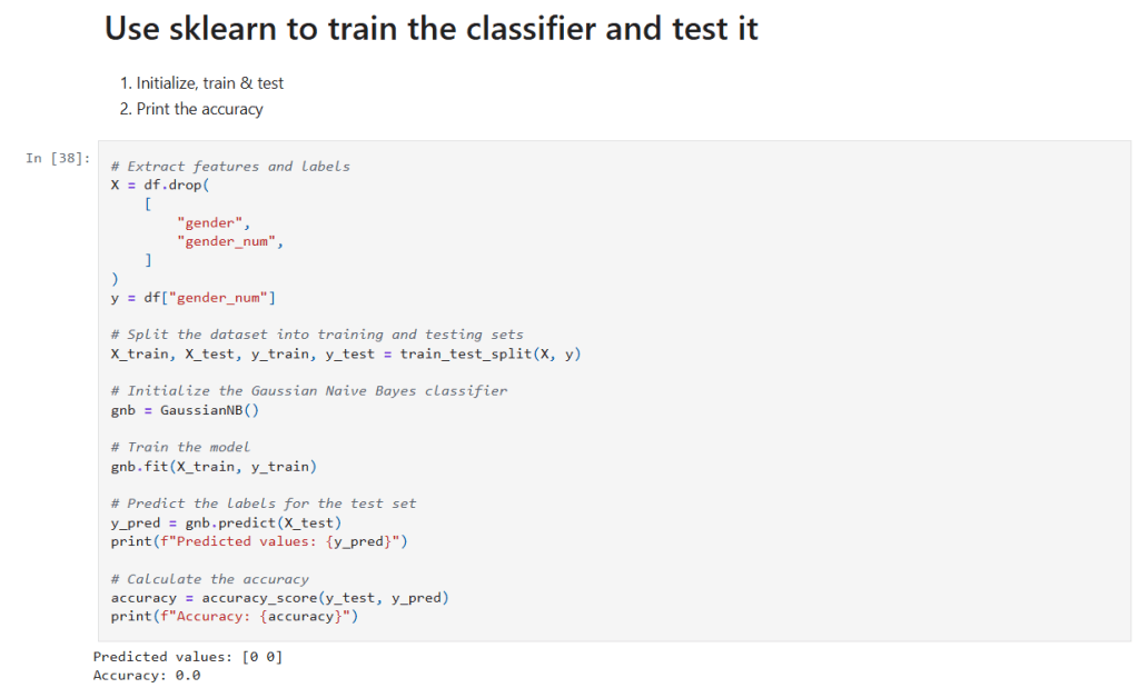
Experimenting With Gaussian Naive Bayes
The heart of this exploration was to see how well a Gaussian Naive Bayes classifier could predict the final math grade based on different selections of features. Naive Bayes, while greatly valued for its simplicity and speed, operates under the assumption that features are independent—a condition that might not fully hold in educational data.
Training and Evaluation Function
To streamline the experiments, I wrote a function that:
- Splits the data into training and testing sets.
- Trains a GaussianNB model.
- Evaluates accuracy on the test set.

In that cell:
- I create a function that:
- Drops unwanted columns.
- Runs 100 training cycles with the given data.
- Captures the accuracy measured from each run and returns the average.
Single and Two column sampling

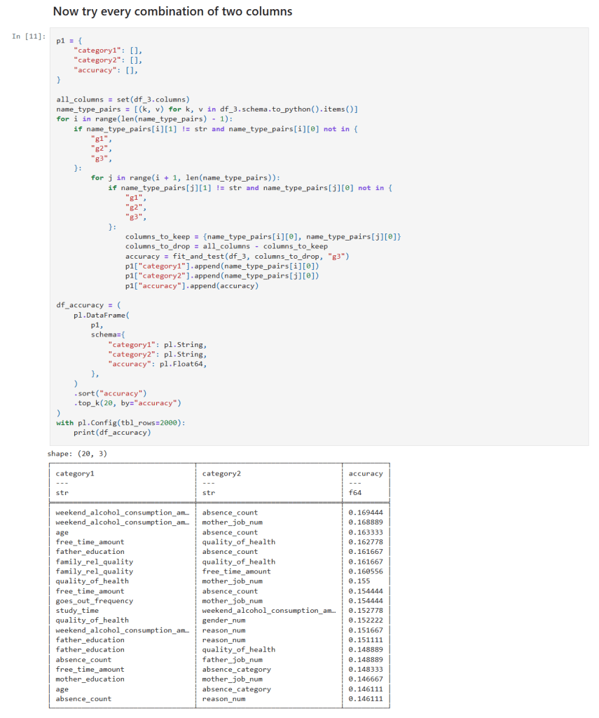
In those cells:
- I get a list of all columns.
- I create loop(s) over the column list and create a list of features to test.
- I call my function to measure the the accuracy of the features at predicting student grades.
Diving Into Feature Combinations
I aimed to assess the predictive power by testing different combinations of features:
- All Columns: This gave the best accuracy of around 22%, yet it was clear that even the full spectrum of information struggled to make strong predictions.
- Handpicked Features: I manually selected features that I hypothesized might be influential. The resulting accuracy dipped below that of the full dataset.
- Individual Features: Evaluating each feature solo revealed that the column indicating whether students planned to pursue higher education yielded the highest individual accuracy—though still far lower than all features combined.
- Two-Feature Combinations: By testing all pairs, I noticed that combinations including weekend alcohol consumption appeared in the top 20 predictive pairs four times, including in both of the top two.
- Three-Feature Combinations: The trend became stronger—combinations featuring weekend alcohol consumption topped the list ten times and were present in each of the top three combinations!
- Four-Feature Combinations: Here, weekend alcohol consumption featured in the top 20 combination results even more robustly—15 times in total.
These experiments showcased one noteworthy pattern: weekend alcohol consumption consistently emerged as a common denominator in the best-performing feature combinations, while weekday consumption rarely made an appearance.
Analysis of the Findings
Several key observations emerged from this series of experiments:
- Predictive Accuracy: Even with the full set of features, the best accuracy reached was only around 22%. This underwhelming performance is indicative of the challenges posed by the dataset and the restrictive assumptions embedded within the Naive Bayes model.
- Role of Alcohol Consumption: The repeated appearance of weekend alcohol consumption in high-ranking feature combinations suggests a potential association—it may capture lifestyle or social habits that indirectly correlate with academic performance. However, it is not a standalone predictor; rather, it seems to be relevant as part of a multifactorial interaction.
- Model Limitations: The Gaussian Naive Bayes classifier assumes feature independence. The complexities inherent in student performance—where multiple social, educational, and psychological factors interact—likely violate this assumption, leading to lower predictive performance.
Conclusion and Future Directions
While the Gaussian Naive Bayes classifier provided some interesting insights, especially regarding the recurring presence of weekend alcohol consumption in influential feature combinations, its overall accuracy was modest. Predicting the final math grade, a multifaceted outcome influenced by numerous interdependent factors, appears too challenging for this simplistic probabilistic model.
Next Steps:
- Alternative Machine Learning Algorithms: Investigating other approaches like decision trees, random forests, support vector machines, or ensemble methods may yield better performance.
- Enhanced Feature Engineering: Incorporating interaction terms or domain-specific features might help capture the complex relationships between social habits and academic outcomes.
- Broader Data Explorations: Diving deeper into other factors—such as study habits, parental support, and extracurricular involvement—could provide additional clarity.
Final Thoughts and Next Steps
This journey reinforced the idea that while Naive Bayes is a great tool for its speed and interpretability, it might not be the best choice for all datasets. More sophisticated models and careful feature engineering are necessary when dealing with some datasets like student academic performance.
The new Jupyter notebook can be found here in my GitHub.
– William